Surfels and Spatial Storage

Introduction

Purpose of this document

The aim of this document is to explain what surfels are, how they are currently being used, and how it could enhance our project. A conclusion can be found at the end of the document. This contains a brief summary of the outcomes of the research and the most important things the reader might want to know about surfels and spatial storage.

Previous research

Our team has never done any research into surfels. Therefore, this document will start from scratch and build upon the fundamentals explained in the first chapter.

Research questions

What are surfels?
What are surfels used for?
How does EA SEED use surfels?
How does Pixar use surfels?
Can we use surfels for our project?
- Time estimation.
- Risk analysis.
- Conclusion.

Definition

Surfels are ‘surface elements’ or ‘surface voxels’ in the volume rendering literature. Others describe it as a zero-dimensional n-tuple with shape and shade attributes that locally approximate an object surface. Objects can be represented by a dense set of points (surfels) holding lighting information.

Why surfels?

Because the team did not have the budget to solve global illumination every frame, some sort of special or temporal accumulation was needed. The budget was roughly 250.000 rays per frame to calculate the global illumination.

When storing light accumulation, there are generally two way to store the data: screen-space and world-space. The advantage of screen-space storage is that the resolution increases when the camera moves closer to a surface. However, this only works really well for static environments. It does not work as well for dynamic scenes as “ghosting” could become visible.

Therefore, the team chose to go with world-space storage for the global illumination accumulation. This is where surfels come into play. Each surfel stores a position, normal, radius, and some animation information. The surfels are persistent. This allows for global illumination accumulation over time.

Surfels can be skinned. This makes it possible to place surfels on animated meshes. Each surfel has a smooth falloff, which gives a uniform look during rendering.

To apply surfels to the screen, a technique similar to rendering deferred light sources. The payload per surfel is just irradiance, no direction.

Surfels are culled using a world-space data structure very much like an octree. Each cell stores a list of intersecting surfels. Each point in space can query the data structure and find all relevant surfels.

EA SEED

Common applications of Surfels are medical scanner data representations, rendering surfaces of volumetric data and real-time rendering of particle systems. Surfels are also used to improve the efficiency of GI (Global Illumination) as Tomasz Stachowiak from EA SEED describes.

In interactive applications like games or game engines, surfels are very useful to store lighting data in. This can make lighting passes much faster since lighting data is already available at areas where surfels are spawned.

Surfel placement

The placement algorithm uses G-buffer information and it’s an iterative hole filler. Starting from calculating the coverage of each pixel by the current surfel set, it should look for pixels with low coverage so it can spawn new surfels in those locations. EA SEED found a way to find those low coverage signals.

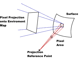
They first divided the screen in tiles (in their case: 16x16 pixels) and for each tile, they find the lowest coverage signal using ‘group atomic sense wave operations’. Then, the surfel is spawned using the G-buffer’s depth and normal data. One thing to take into account is the pixel’s projected area. When you’re facing a wall, you don’t want a lot of surfels spawning there, based on only the screen (16x16)-tiles, because the distribution of the surfels isn’t the same as it is for objects that are further away.

A projected pixel area is exactly what it says. Take the images to the right as examples. The image is rendered on a window of 7x5 pixels. Each green pixel covers a part of the sphere, which is the projected area. The lower image shows it even better. The projected area of the pixel can be seen on the surface and determines the projected area of the pixel.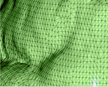

So, if the projected area of the pixel is too small, the surfel placement algorithm takes this into account and won’t spawn a lot of surfels very close to each other. It will equally distribute the surfels just like it should on objects further away.

This process of spawning new surfels at poor coverage areas happens every frame. A newly spawned surfel will compute more samples than an already spawned surfel to reduce noise. A spawned surfel will roughly compute one path trace per frame. When a path trace is traced and hits a surfel, it uses the lighting data of that surfel, reuses its own lighting data from the previous frame and amortizes the extra bounces over time to calculate the new/improved lighting data.

This algorithm is much closer to radiosity than path tracing, but the visual result is quite similar.

Global Illumination

Surfels can be used in a lot of applications/techniques. This can be in medical applications to store regional data of scans or in interactive applications with interactive GI. Surfels are really useful for GI, because they store lighting data of a small area, which the GI can find and ‘easily’ render a scene with interactive GI.

One method to implement this is the Monte Carlo method. However, this is not good practice to use in interactive applications with a dynamic scene. The Monte Carlo method does a hard reset everytime something in the scene changes. This shows weird artifacts (use can see the lighting data changing/calculating) on models as soon as something changes its orientation.

Instead, you can use a modified exponential means estimator. The formulation is very similar to the formulation of plain Monte Carlo. However, the blending factors are defined in another way. Exponential averaging the weights for a new sample is constant (usually set to a small value) so that the input variance will not be jarring in the output. It’s easy to notice that if the input doesn’t have high variance, then the output won’t either. This is potentially wasting convergence speed. You can potentially use a higher blending factor when detecting that variance is low.

The specifics of EA SEED’s integrands are changed dynamically all the time. You need to figure this out from the scene by using short terms statistics of mean and variance to inform the long-term blending factors. That gives the idea of the plausible range of values that the sample should fall into. When you create new ones, they should follow them like 2σ, for example.

When they start to drift you can increase the blending factor.

Eventually, this gives a better effect than the Monte Carlo method, because this method exponentially changes to simulate correct GI.

High-level implementation

There are at least two ways to implement surfels in spatial storage. Either using LDI/LDC trees or the Pica Pica approach: using screen-space to determine where to spawn surfels stored in a tree very similar to an Octree. Since that is already described in the [EA SEED]{.underline} section, I’ll only go over the LDI/LDC tree.

LDI/LDC Tree

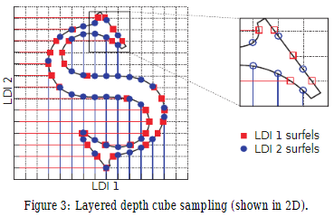
Hanspeter Pﬁster, Matthias Zwicker, Jeroen van Baar, and Markus Gross explain this tree really well in their research document[1]. LDC stands for Layered Depth Cube and LDI stands for Layered Depth Image. A LDC consists of three LDI’s. This describes the cube.

They use ray-tracing to create these three LDI’s. The LDI’s store multiple surfels along each ray, one for each ray-surface intersection point.

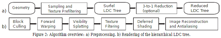
This tree is also based on an Oct-tree. Each octree node stores one LDC, which is called a ‘block’. The whole tree is also known as a LDC-tree. On this tree, a ‘3-to-1 reduction’-step is performed and reduces the LDC’s to single LDI’s on a block-by-block basis. To increases the rendering speed.

The rendering pipeline projects the blocks to screen space using perspective projection and is accelerated by block culling and some other techniques (Forward Warping, Visibility Splatting etc. (the pipeline can be seen in the image below and is described in the PDF of Pfister, Zwicker, van Baar, and Gross)[1]).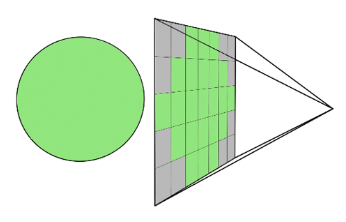

At each ray intersection point, a surfel is created with floating point depth and other shape- and shade- (if implemented) properties.

To reduce storage and rendering time it is useful to optionally reduce the LDC’s to one LDI on a block-by-block basis. Reducing the amount of LDI’s per block is pretty straightforward. Get all intersection points of the sample rays (where the sample rays of the three LDI’s intersect). These intersection points are used by Nearest Neighbor interpolation: sampled surfel positions find the nearest intersection point and get bound to that. Although, a more sophisticated filter, like Splatting, could easily be implemented.

This means that the quality of the surfels locations depends on the density of the sampled rays per LDI’s.

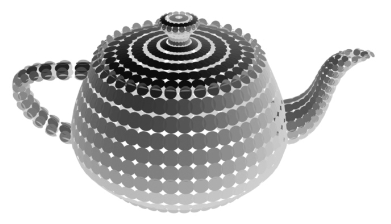
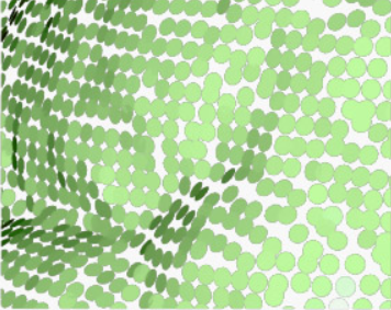
Point-based approximate color bleeding

Point-based color bleeding is a global illumination technique. It makes use of a surfel cloud to represent the surface of an object. A surfel cloud is very similar to a point cloud. However, the surfel cloud consists out of polygonal meshes with overlapping surfels, instead of just points.

In point-based approximate color bleeding, surfels are used to represent the direct illumination of the scene. Each surfel stores a position, normal, color, and radius. When calculating the color bleeding value of a specific point, the closest surfels within a certain radius are used to determine the color bleeding value.

Polygonal mesh Surfel "mesh"

Generating the surfels

Using surfels for global illumination requires at least two passes. The first pass is used to generate the surfel surfaces for the entire scene. Each surfel that is generated should store the direct illumination data, this includes shadows. The more surfels on a surface, the better the color bleeding will look (having more data points means more there is more color information available for a given point in space).

For static geometry, the first pass would only have to be executed once for the entire application, because it will never change. Once dynamic objects are added, the spatial partitioning structure will have to be updated as the object moves through 3D space.

Since the surfel representation of the scene could potentially become huge, it would make sense to use some kind of spatial partitioning structure such as an octree. This will help speed up the second pass, as that one will have to query all surfels that are close to a point in space.

Calculating color bleeding

The algorithm itself is relatively simple. Each point that needs to be rendered checks the surrounding area and queries the data from all surfels in that section of the octree. The surfels from the surfel cloud are used to generate a cube map surrounding the point. This cube map can then be used to calculate the color that bleeds onto the point based on the normal of the surface. All pixels in the color map are multiplied by the reflectance function (BRDF) and added to the current direct illumination color. The result is the color bleeding that that point.

If the surfel resolution is low, the cubemap will only use a few colors, which will not give great color bleeding. Experimentation may be needed to find the optimal number of surfels per surface area.

Optimizing the surfel color looking can be done by combining a cluster of distant points into a single color. Since they are “far” away, their colors can be combined without any real visual differences. There may be cases where the color bleeding difference is minimal, this color can be interpolated to save some processing power.

In case the point querying surfels is really close to a surfel, ray tracing it may be a solution. That way, one surfel can be sampled multiple times.

One of the issues that may arise when averaging colors in a radius is that it does not take occlusion into account. Occluding surfels should block other surfels and there, prevent those from contributing to the final image. The way Pixar solved this is by rasterizing the surfels as if they are viewed from the point that is being calculated. This will give a good color map of which surfels contribute to the final color output.

Of course, the result still needs to be saved to a cube map per point that is being evaluated, but that is not any different from what we have seen before. The only difference this time is that colors that could contribute to the final color are rasterized before applying them to the cube map.

Examples from the Pixar "point-based color bleeding" presentation.

Conclusion

Compared to EA SEED’s approach, the LDC-tree would take much more performance. It traces rays to find surfels locations, while EA SEED just uses the G-buffer, which is much faster than building an Octree from traced rays.

Surfels are extremely useful for point-based approximate color bleeding. Surfels are disks in world-space that store direct lighting information (including shadows), a normal, a position, and the radius of the disk. This information can then be queried to calculate the color bleeding values for a point in space.

Generating surfels on static geometry only has to be done once, but dynamic geometry force the spatial partitioning data structure to update (surfels have to move with the geometry). EA SEED took this a step further and added on-the-fly surfel generation and skinning.

Risk analysis

Surfels provide a relatively simple solution to approximating color

bleeding.
Lots of resources out there that describe the theory and

implementation.
Surfel cloud resolution directly impacts performance, the resolution

can be lowered if more processing power is needed elsewhere.

Surfel generation could take a long time.
Skinning surfels like EA SEED could pose a real challenge.
Surfels by themselves are not new, the EA SEED application is.

Time estimation

Taking my experience with this subject and knowledge into account, I think the implementation of Surfels will take around 6-8 weeks (so about 1 school-block (8 weeks)), however, there is a student on Twitter who has shown his EA SEED-like surfel generation. This took him approximately 4 weeks.

A lot of research is still needed and implementations are hard to find. It also depends on who will implement it (how much knowledge that person has) and on the architecture that is/has to be built with it.

This estimation is only aimed at surfels. Using the surfels to implement something like Global Illumination will take even longer. I would say, something like 2-4 weeks since you already have the surfel implementation.

EA SEED is, however, always ready to answer questions on Twitter. This usually wouldn’t take much longer than one day.

References

Referenced articles

[1] Surfels: Surface Elements as Rendering Primitives PDF - Hanspeter Pﬁster, Matthias Zwicker, Jeroen van Baar, and Markus Gross

[https://www.researchgate.net/publication/2462148_Surfels_Surface_Elements_as_Rendering_Primitives]{.underline}

Unreferenced articles

What is a Spatial Database? - Definition from Techopedia

[https://www.techopedia.com/definition/17287/spatial-database]{.underline}

Spatial Database - Wikipedia.org

[https://en.wikipedia.org/wiki/Spatial_database]{.underline}

DD2018: Tomasz Stachowiak - Stochastic all the things: raytracing in hybrid real-time rendering

[https://www.youtube.com/watch?v=MyTOGHqyquU]{.underline}

Surfels: Surface Elements as Rendering Primitives - Hanspeter Pﬁster, Matthias Zwicker, Jeroen van Baar, and Markus Gross

[https://graphics.ethz.ch/research/past_projects/surfels/surfels/index.html]{.underline}

Layered Depth Images - Harvard Library

[https://dash.harvard.edu/bitstream/handle/1/2640599/Gortler_LayeredDepth.pdf?sequence=2&isAllowed=y]{.underline}

Surfel - Wikipedia

[https://en.wikipedia.org/wiki/Surfel]{.underline}

Introduction to Ray Tracing: a Simple Method for Creating 3D Images - Implementing the Raytracing Algorithm

[https://www.scratchapixel.com/lessons/3d-basic-rendering/introduction-to-ray-tracing/implementing-the-raytracing-algorithm]{.underline}

12. Textures - Environmental Mapping

[https://www.csee.umbc.edu/~rheingan/435/pages/res/gen-12.Textures-single-page-0.html]{.underline}

Bunnell, M. Dynamic Ambient Occlusion and Indirect Lighting (2005, February 2). Retrieved from

[http://downloads.gamedev.net/pdf/Pharr_ch14.pdf]{.underline}

Christensen, P. Point-Based Global Illumination for Movie Production (2010). Retrieved from

[https://graphics.pixar.com/library/PointBasedGlobalIlluminationForMovieProduction/paper.pdf]{.underline}

Christensen, P. Point-Based Approximate Color Bleeding (n.d.). Retrieved from

[https://graphics.pixar.com/library/PointBasedColorBleeding/paper.pdf]{.underline}