Bilateral Filtering
Foreword
Purpose of this document
We took a lot of inspiration from the research done by EA SEED with Pica Pica on real-time raytracing [2]. For cleaning up the noise that is exhibited by raytraced reflections with low sample counts they use a variety of techniques. The clean up consists out of spacial reconstruction, temporal accumulation, bilateral filtering and temporal anti-aliasing. In this document, I’ll share my findings on bilateral filtering to streamline the implementation later in the project and to assist the team’s planning. To achieve this I heavily relied on the paper that first proposed this technique [1].
Why bilateral filtering
Traditional low pass filtering works by computing a weighted average of pixels based on the distance from the center. This assumes that the color varies slowly over time which works well with noise as the noise doesn’t have a significant impact on the weighted average. Yet this assumption fails at edges where drastic color changes are to be expected which. This leads to blurred edges as the filter has no notion of changes in color. Bilateral promises to fix this by taking the color similarity into the weighted average leading to edges with drastically changing colors being preserved. The pictures below are from Pica Pica with the first one before and the second one after bilateral filtering. Notice the severe reduction in noise specifically visible inside the tunnel and on the boxes. All without reducing the crispness of the edges.
Limitations
Computation time
Bilateral filtering uses a Gaussian function for the distance and similarity weights. This means that in the purest form every pixel would contribute to the weighted average meaning that every pixel has to be sampled for every output pixel meaning the computation time would scale exponentially with screen size. Possible fixes will be suggested later in this document.
RGB color accuracy
Most of the research done in the reference paper has been done initially using grayscale images as these colors scale perfectly linear. With multiband images, it becomes a different story as filtering every one of the color channels separately doesn’t yield the same visual differences as intended. The fix mentioned in the aforementioned paper is to use the SIElab color scheme as this is uniform with human color perception thus making the filtering look a lot more natural than when filtering traditional RGB color bands.
Added blur
The purpose of bilateral filtering is to either compress textures by decreasing the amount of detail or to remove noise from an image. While this is what we need for denoising reflections it does mean that finer details might fade away and the picture might seem blurry. It is described by Tomasz Stachowiak from EA SEED as a dumb, blunt instrument and should be used sporadically. This ties in neatly with the computation problem and a solution for both issues will be proposed further on this document
Technical details
Mathematical definition The formula for a filtered pixel as proposed by Tomasi and Manduchi is written the clearest on Wikipedia [6] but the same formula is used various papers [1, 3, 4, 5]

Where the weight of all the pixels used for normalization is
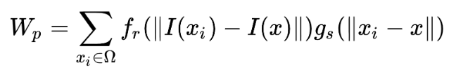
For the rest of the variables
is the filtered image
is the input image
is the texture to denoise centered at x
are the coordinates of the pixel currently being filtered
is the range kernel for color similarity
is the range kernel for geometric closeness
When we use Gaussian functions for and we can define the weight of a pixel as
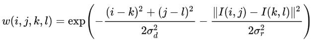
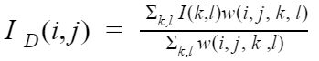
In this, i and j are the coordinates of the input pixel and k and l are coordinates of a nearby pixel. and are the standard deviations of the function which can be used to alter the filtering characteristics. Once you apply this weight to the equation mentioned before you can get the filtered pixel with the function on the bellow.
Optimizations
Limiting the kernel
In the equations mentioned earlier, the weight of every pixel in the texture is used to determine a filtered pixel. In truth, it could be stated that the pixels outside of the standard deviation used in the geometric closeness weight can be neglected to the final result of a filtered pixel. If we limit the sampling of neighboring pixels to only those within the standard deviation we get a much smaller kernel which will massively decrease the time needed for filtering.
Pica Pica’s variable kernel
EA seed uses an interesting trick to limit the kernel to reduce blur. During the temporal accumulation pass, they calculate a variance which tells the amount of noise in certain areas of the texture. The kernel then is adjusted based on this variance which means that on simple area’s with very little noise the filter won’t be nearly as aggressive and much more detail will be preserved. Yet in smaller nooks and crannies where there might be significant amounts of noise the filter will do whatever it takes to remove the noise with will lead to a blurrier result.
Conclusion
While Bilateral filtering is not a magical instrument that removes all the noise from a scene, it is a great filtering technique for our purpose when applied correctly. A feel like a simple version can be implemented really quickly with the formulas described here. This simple version will likely contain a fixed kernel and apply the filter with the same strength over the entire image. After this, the next step would be to make the kernel size respond to the amount of noise that is to be filtered. This implementation is relying on the variance calculated during the temporal accumulation which I have no knowledge on the requirements to calculate this. I believe the first step should be done within a single working day and once the variance per pixel is available I believe it would be done in a similar or shorter timeframe but tweaking this value will require additional research.
References
- [1] C. Tomasi, R. Manduchi, in Sixth International Conference on Computer Vision (IEEE Cat. No.98CH36271)(Narosa Publishing House; http://ieeexplore.ieee.org/document/710815/), pp. 839–846.
- [2] Tomasz Stachowiak, in Digital Dragons 2018 https://www.ea.com/seed/news/seed-dd18-presentation-slides-raytracing
- [3] F. Banterle, M. Corsini, P. Cignoni, R. Scopigno, A low-memory, straightforward and fast bilateral filter through subsampling in spatial domain. Computer Graphics Forum. 31, 19–32 (2012). http://doi.wiley.com/10.1111/j.1467-8659.2011.02078.x
- [4] P. Kornprobst, Limitations? - A Gentle Introduction to Bilateral Filtering and its Applications(2007; http://people.csail.mit.edu/sparis/bf_course/slides/09_limitations.pdf).
- [5] A. Adams, J. Baek, M. A. Davis, Fast high-dimensional filtering using the permutohedral lattice. Computer Graphics Forum. 29, 753–762 (2010). http://www.ncbi.nlm.nih.gov/pubmed/16473905
- [6] Bilateral filter, Wikipedia https://en.wikipedia.org/wiki/Bilateral_filter